How to Avoid Unexpected Year-end Sales Comp Budget Breakers

“How did you manage to overspend your sales compensation budget?”

There’s a question sales leaders do not want to hear from their CFO. Unfortunately, this prickly question seems to come up too often, and too late. There is very little anyone can do at the end of the plan year to remedy a sales compensation budget overrun. Likewise, underspending the sales compensation budget may carry negative implications, such as frustrated sales personnel and embattled first-line sales managers. Sales management needs to correctly cost the incentive plan at the outset of the plan year and manage it accordingly. This work is part art, part science. There are four primary factors that drive the estimated sales compensation budget.

1. Payout curves
2. Adjusted value multipliers
3. Expected performance distributions by metric
4. Open territories

Missing the mark on any one of these four factors can cause unanticipated variance either below or above expected budget. A cost model that incorporates and links all four components will ensure costs are fully aligned with the budget. The “art” of cost modeling requires the modeler to be facile at linking all four variables and modifying their impact based on the forecasted performance of the sales organization. As a reminder, there can be other variables that impact the budget post plan implementation such as: poorly administered plans, crediting rules, discretionary bonuses, SPIFFs, etc.

Payout Curves

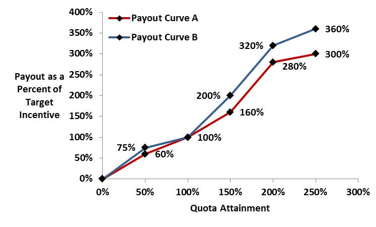
The payout curve for each metric describes the pay schedule depending on dollars/units sold or quota achieved. After constructing the payout curve, calculate both individual and aggregate costs based on expected performance levels by individual. Construct a cost model to reference the expected performance for each metric, and then return the associated payout for that metric based on the payout curve. For example, the cost of Payout Curve A will be less than Payout Curve B since it has a shallower slope (see Figure 1).

Figure 1: Payout Curve Illustrations

Adjusted Value Multipliers (AVMs)

AVMs change the payout value of a sale based on a factor added or subtracted within the plan design reflecting management’s sales preferences. For example, instead of having an incentive par value of $1 for each dollar of sale, the adjusted value might be $1.20, providing a 20% premium for the sale of the preferred product.

Use the Adjusted Value Multiplier Index (AVMI) to understand how the AVMs impact payouts versus actual financial performance. Figure 2 illustrates how to calculate the AVMI. Calculate the AVMI based on the AVMs and the expected aggregate annual financial forecast by product type. If the AVMI is more than 1.00, costs will increase. Conversely, an AVMI that is less than 1.00 will lower plan costs.

Figure 2: Adjusted Value Multiplier Index Illustration (AVMI)

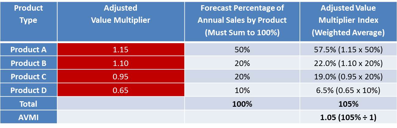
Construct the model to allow changes to the AVMs (cells in red). It’s best to set the adjusted value multipliers to keep the AVMI within an acceptable +/- .05 variance of 1.0 (.95 to 1.05).

The next step is to adjust the expected individual quota attainment based on the AVMI. For example, Sales Rep 1 achieved 100% attainment of their financial quota. However, the 100% attainment is adjusted (up in this case) based on the previously calculated AVMI of 1.05 to 105%. Payouts will be based on 105%, not 100% quota attainment. This will result in a higher incentive payout increasing overall plan costs.

Expected Performance Distribution

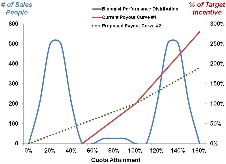
A typical approach involves the use of historical data to depict the shape and dispersion of expected performance. Management can improve the accuracy of the cost model by applying the payout curve to the expected performance distribution (see Figure 3). Modeling different performance curves will improve forecast accuracy. For instance, modeling a bi-modal distribution where 50% of sales personnel fall below quota and the other 50% of sales personnel perform above quota (see blue performance curve below) results in a very different cost envelope. The red payout curve represents the current incentive formula. In this scenario, nearly 50% of the plan participants will not earn an incentive because they are below the threshold. The current comp plan could be attributing to the bi-modal results. One approach to correct this is to lower the threshold and reduce excellence payout levels (see green payout curve).

Figure 3: Adjusting Payout Curves to Expected Quota Performance Illustration

A final point on using historical data: Typically, the historical performance will not equal 100% in aggregate—it might be higher or lower. To correct for this, index the data to shift actual individual performance to obtain 100% aggregate attainment. For example, if last year’s overall performance was 105% of quota, shift the distribution to the left by adjusting each individual attainment level by 0.952 (100% ÷ 105%). The shape of the curve stays constant but is indexed from 105% to establish 100% aggregate attainment.

If historical data is not available, then the cost modeler should obtain input from sales, marketing and finance management on the expected performance distribution.

Open Territories

Employee turnover will temporarily create unfilled territories. Unfilled territories reduce plan costs because there is no salesperson to receive sales credit. The best predictor of unfilled territories is to analyze historical turnover rates. Additionally, solicit input from sales and field human resources to understand if there are any plan changes or economic factors that may require adjustments to turnover rate assumptions.

Once the turnover rate and the estimated duration of the empty territory are determined, calculate the Open Territory Index (OTI). Use this calculation to determine the OTI: (Planned FTEs – Employee Turnover FTEs – Unfilled Territories FTE) ÷ Planned FTEs

For example, assume aggregate plan costs are $2.8 million based on the prior three factors (payout curve, AVMI, quota distribution). Assume an OTI of .90 based on the equation above. The final adjusted cost—applying OTI—would be $2.52 million ($2.8 million x 0.90).

Incorporating All Four Factors

It’s not enough to get just one cost adjustment factor correct. Effectively forecasting the sales compensation budget requires incorporating many factors. Thus, when building your model, ensure you have the ability to:

1. Adjust the payout curve inflection points.
2. Change the adjusted value multipliers by product or account to reduce or increase the AVMI.
3. Modify the quota performance from normal low standard deviation to normal high standard deviation or bi-modal.
4. Increase or decrease the total cost based on the OTI.

Did you correctly forecast your sales compensation budget this past fiscal year? Are you confident in your forecast for the current fiscal year? If you are interested in learning more about forecasting your sales compensation costs, please visit our Sales Compensation Practice page.